Modelling Historical Data for an All-In-One Fund ETF

VDAL is a new all-in-one fund ETF created by Vanguard, brought out by popular demand for a VDHG ETF alternative without the bonds. Although this new ETF is very promising, its historical data is limited as it was only recently released. Through analysis of its underlying holdings, we can predict and extend this data decades into the past.

Note

Because this process is quite long and technical, you can skip ahead to the final result by navigating through the sidebar. The rest of the article (which explains methodology and provides all code) is optional and is not designed to be read on mobile.

Packages, configurations, and functions used

Packages

import datetime as dt
import numpy as np
import pandas as pd
import pandas_datareader.data as web
import matplotlib.pyplot as plt
import matplotlib.ticker as mtick
import matplotlib.patches as patches
import matplotlib.colors as mcolors
import yfinance as yf
from sklearn.metrics import r2_score
from sklearn.linear_model import LinearRegression
from matplotlib.ticker import LogLocator, FuncFormatter
from matplotlib.ticker import ScalarFormatter

Configurations

plt.rc("figure", labelsize="x-large", autolayout=True, figsize=(4, 3))

Functions

def set_offset_from_first_valid_index(df, col, offset, y):
    first_valid_index = df[col].first_valid_index()
    offset_from_first_valid_index = df[col].index.get_loc(first_valid_index) + offset
    df.loc[df.index[offset_from_first_valid_index], col] = y

def normalised(x):
    x = x.ffill().dropna().pct_change(fill_method=None)
    x = (1 + x).cumprod()
    x.iloc[0] = 1

    return x

def normalise_stock_performance(df, rebase_stock=None):
    # default to youngest stock
    if rebase_stock == None:
        rebase_stock = (
            df.apply(lambda x: x.first_valid_index())
            .sort_values(ascending=False).index[0]
        )
        
    df = df.copy()

    # normalise each column individually
    for stock in df.columns:
        df[stock] = normalised(df[stock])
        
    # scale stocks relatively
    rebase_date = df[rebase_stock].first_valid_index()
    for stock in df.columns:
        rebase_value = df[stock].loc[rebase_date]
        df[stock] = df[stock] / rebase_value

    return df

def plot_correlation(df, actual, predicted, actual_label=None, predicted_label=None):
    if actual_label == None:
        actual_label = actual

    if predicted_label == None:
        predicted_label = predicted
        
    plot_df = df[[actual, predicted]]
    plot_df = plot_df.dropna()
    plot_df = normalise_stock_performance(plot_df)
    
    y1 = (plot_df.pct_change(fill_method=None) + 1).dropna()
    y1 = y1.rolling(30).apply(lambda x: x.prod()).dropna()
    y1 -= 1
    y_true = y1[actual]
    y_pred = y1[predicted]
    r2 = r2_score(y_true, y_pred)

    x2 = np.array(y_true).reshape(-1, 1)
    y2 = np.array(y_pred)
    model = LinearRegression()
    model.fit(x2, y2)
    x_fit = np.linspace(x2.min(), x2.max(), 100).reshape(-1, 1)
    y_fit = model.predict(x_fit)
    slope = model.coef_[0]
    intercept = model.intercept_

    fig, axs = plt.subplots(1, 2, figsize=(8, 3))
    
    axs[0].plot(plot_df[actual])
    axs[0].plot(plot_df[predicted])
    axs[0].set_title("Total Return (%)")
    axs[0].legend([actual_label, predicted_label])
    axs[0].yaxis.set_major_formatter(FuncFormatter(lambda x, _: f"{100 * (x - 1):.0f}%"))
    
    axs[1].plot([y_true.min(), y_true.max()], [y_true.min(), y_true.max()])
    axs[1].plot(x_fit, y_fit)
    axs[1].scatter(y_true, y_pred, s=1, color=mcolors.TABLEAU_COLORS["tab:orange"], zorder=2)
    axs[1].text(0.1, 0.9, f"R2: {r2:.2f}", transform=axs[1].transAxes)
    axs[1].text(0.1, 0.8, f"y = {slope:.2f}x + {intercept:.2f}", transform=axs[1].transAxes)
    axs[1].set_title(f"30-Day Returns: {actual_label} vs. {predicted_label}")
    axs[1].xaxis.set_major_formatter(mtick.FuncFormatter(lambda x, _: f"{100 * x:.0f}%"))
    axs[1].yaxis.set_major_formatter(mtick.FuncFormatter(lambda x, _: f"{100 * x:.0f}%"))

    fig.autofmt_xdate()
    
    plt.show()

Downloading and preparing the data

stocks = ["VDAL.AX", "VDHG.AX"]
stocks += ["VAS.AX", "VGS.AX", "VGAD.AX", "VISM.AX", "VGE.AX"]
stocks += ["IOO.AX", "STW.AX", "IEM.AX"]
stocks += ["IOO", "EWA", "EEM"]
stocks += ["^SP500TR"]
df_orig = yf.download(stocks, period="max", group_by="ticker", auto_adjust=False)
aud_usd = web.DataReader("DEXUSAL", "fred", start=dt.datetime(1900, 1, 1))

df = df_orig.copy()
df = df.xs("Adj Close", axis=1, level=1)
df["AUDUSD=X"] = aud_usd
df["USDAUD=X"] = 1 / df["AUDUSD=X"]

Looking at VDAL’s holdings

From VDAL’s fact sheet, we can see its target asset allocation is as follows:

Asset	Target (%)
Australian Shares	40
International Shares	29.5
International Shares (Hedged)	18
International Small Companies	7
Emerging Markets Shares	5.5

We can look at various ETFs and indices to model this allocation. However, as you will soon see, the further into the past we go, the more we need to compromise on accuracy. To get the best of both worlds, we will create multiple models with varying trade-offs between accuracy and length. Afterwards, we can then append them all together in order of accuracy.

Model A: Weighted Return of Component ETFs

For our first model, let’s look at the actual holdings of VDAL. The above allocation specifically corresponds to five Vanguard ETFs: VAS, VGS, VGAD, VISM, and VGE. All five of these ETFs are much older than VDAL, allowing us to highly accurately model VDAL prior to its inception date.

Model A will be created through the combined return of the five component ETFs, weighted accordingly by their target allocations:

df["model_a"] = (
    0.40 * df["VAS.AX"].pct_change(fill_method=None) +
    0.295 * df["VGS.AX"].pct_change(fill_method=None) +
    0.18 * df["VGAD.AX"].pct_change(fill_method=None) +
    0.07 * df["VISM.AX"].pct_change(fill_method=None) +
    0.055 * df["VGE.AX"].pct_change(fill_method=None)
)

df["model_a"] = (df["model_a"] + 1).cumprod()
set_offset_from_first_valid_index(df, "model_a", -1, 1)

plot_correlation(df, "VDAL.AX", "model_a", "Actual", "Model A")

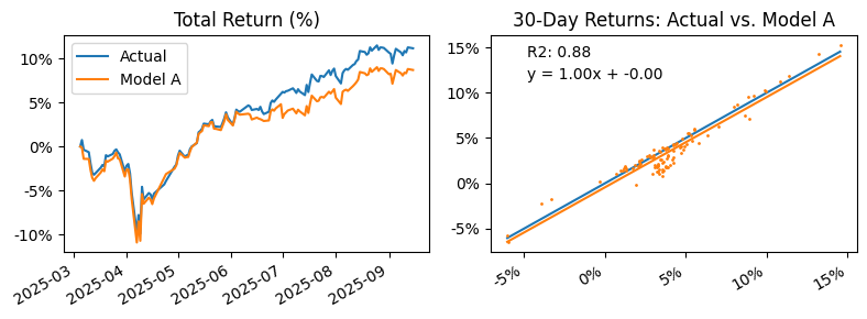
Model A has a strong correlation to the original, giving high confidence that the predicted data past VDAL’s inception date is reliable.

Model B: Absorbing VISM into VGS

When looking at the five component ETFs, VISM’s inception date is significantly later than the rest. If we were to substitute VISM in our next model, we can extend the data a further four years.

I chose to absorb VISM (International Small Cap) into VGS (International Large/Mid Cap), justifying that the two should perform similarly to due to their similar regional exposure. Additionally, because VISM only makes up a small fraction of the total allocation, any minor difference caused by this substitution should turn negligible.

Let’s first test our assumptions by comparing the two components:

plot_correlation(df, "VISM.AX", "VGS.AX", "VISM", "VGS")

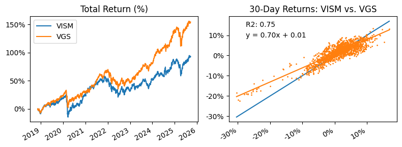
As thought, VISM and VGS share a moderate correlation.

Let’s now test the effect of this substitution in model B:

df["model_b"] = (
    0.40 * df["VAS.AX"].pct_change(fill_method=None) +
    (0.295 + 0.07) * df["VGS.AX"].pct_change(fill_method=None) +
    0.18 * df["VGAD.AX"].pct_change(fill_method=None) +
    0.055 * df["VGE.AX"].pct_change(fill_method=None)
)

df["model_b"] = (df["model_b"] + 1).cumprod()
set_offset_from_first_valid_index(df, "model_b", -1, 1)

plot_correlation(df, "VDAL.AX", "model_b", "Actual", "Model B")

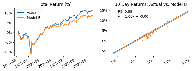
We can see that our assumptions were correct. No significant change in correlation was observed from this substitution.

Model C: Substituting Components with Older ETFs

Similarly, further data can be obtained by substituting components with entirely different older alternatives that have similar regional exposure:

• VGS (International Large/Mid Cap) with IOO (International Top 100).

• VAS (Australian Shares) with STW (Australian Top 200)

• VGE (Emerging Markets Shares) with IEM (Emerging Markets Shares)

VGAD (International Large/Mid Cap Hedged) is a little bit more tricky as there is no simple currency hedged replacement. We can do our best by modelling a hedged version of IOO by tying it to the performance of AUD/USD:

df["IOO_hedged"] = df["IOO.AX"] * df["AUDUSD=X"]

Now let’s look at how each component is correlated to their corresponding substitution:

plot_correlation(df, "VGS.AX", "IOO.AX", "VGS", "IOO")
plot_correlation(df, "VGAD.AX", "IOO_hedged", "VGAD", "IOO Hedged")
plot_correlation(df, "VAS.AX", "STW.AX", "VAS", "STW")
plot_correlation(df, "VGE.AX", "IEM.AX", "VGE", "IEM")

All substitutes have strong correlations with their original. Let’s now put it together and construct model C:

df["model_c"] = (
    0.40 * df["STW.AX"].pct_change(fill_method=None) +
    (0.295 + 0.07) * df["IOO.AX"].pct_change(fill_method=None) +
    0.18 * df["IOO_hedged"].pct_change(fill_method=None) +
    0.055 * df["IEM.AX"].pct_change(fill_method=None)
)

df["model_c"] = (df["model_c"] + 1).cumprod()
set_offset_from_first_valid_index(df, "model_c", -1, 1)

plot_correlation(df, "VDAL.AX", "model_c", "Actual", "Model C")

Model C’s correlation remains strong to the original despite the more drastic changes.

Model D: Substituting Components with Older US-based ETFs

In model C, we dealt only with ETFs available on the Australian exchange. But by extending our search to international exchanges such as the US, we can find even more data.

Because we are now looking at the US exchange, we need to factor in currency fluctuations. Much like how we simulated currency hedging in the previous model, we can do the same here to model each ETF as if on the Australian exchange. We also shift the data by one day to adjust for the time zone difference.

df["EWA_USDAUD"] = (df["EWA"] * df["USDAUD=X"]).shift(1)
df["IOO_USDAUD"] = (df["IOO"] * df["USDAUD=X"]).shift(1)
df["EEM_USDAUD"] = (df["EEM"] * df["USDAUD=X"]).shift(1)

plot_correlation(df, "VGS.AX", "IOO_USDAUD", "VGS", "IOO")
plot_correlation(df, "VGAD.AX", "IOO", "VGAD", "IOO ")
plot_correlation(df, "VAS.AX", "EWA_USDAUD", "VAS", "EWA")
plot_correlation(df, "VGE.AX", "EEM_USDAUD", "VGE", "EEM")

Here the correlation score begins to suffer, though still remains relatively strong. Let’s now construct model D:

df["model_d"] = (
    0.40 * df["EWA_USDAUD"].pct_change(fill_method=None) +
    (0.295 + 0.07) * df["IOO_USDAUD"].pct_change(fill_method=None) +
    0.18 * df["IOO"].pct_change(fill_method=None) +
    0.055 * df["EEM_USDAUD"].pct_change(fill_method=None)
)

df["model_d"] = (df["model_d"] + 1).cumprod()
set_offset_from_first_valid_index(df, "model_d", -1, 1)

plot_correlation(df, "VDAL.AX", "model_d", "Actual", "Model D")

Model E: Removing Emerging Markets

At this point we have exhausted possible substitutions. The next step to extend the data then is to simply look at removing the younger components. By removing EEM and absorbing its allocation into the remaining components, model E extends the data a further three years:

df["model_e"] = (
    0.40/0.945 * df["EWA_USDAUD"].pct_change(fill_method=None) +
    (0.295 + 0.07)/0.945 * df["IOO_USDAUD"].pct_change(fill_method=None) +
    0.18/0.945 * df["IOO"].pct_change(fill_method=None)
)

df["model_e"] = (df["model_e"] + 1).cumprod()
set_offset_from_first_valid_index(df, "model_e", -1, 1)

plot_correlation(df, "VDAL.AX", "model_e", "Actual", "Model E")

Model F: Substituting International Shares with the SP500

Although substituting the entire international allocation for the SP500 seems drastic, this may not be case. The US takes up roughly 75% of the developed world’s market cap, meaning we are still retaining a large portion of the international share movement.

The SP500 data will be split into two to cover the hedged and non-hedged components, adjusting for timezone and currency:

df["SP500"] = df["^SP500TR"].shift(1)
df["SP500_USDAUD"] = (df["^SP500TR"] * df["USDAUD=X"]).shift(1)

Then we can compare it to our original VGS and VGAD components:

plot_correlation(df, "VGS.AX", "SP500_USDAUD", "VGS", "IOO")
plot_correlation(df, "VGAD.AX", "SP500", "VGAD", "IOO Hedged")

Remarkably similar considering the perceived nature of the change.

Now we construct model F:

df["model_f"] = (
    0.40/0.945 * df["EWA_USDAUD"].pct_change(fill_method=None) +
    (0.295 + 0.07)/0.945 * df["SP500_USDAUD"].pct_change(fill_method=None) +
    0.18/0.945 * df["SP500"].pct_change(fill_method=None)
)

df["model_f"] = (df["model_f"] + 1).cumprod()
set_offset_from_first_valid_index(df, "model_f", -1, 1)

plot_correlation(df, "VDAL.AX", "model_f", "Actual", "Model F")

Model G: Removing Australian Shares

In model G, to further squeeze out as much data as possible, we remove the Australian share component and leave solely behind the adjusted SP500 data.

df["model_g"] = (
    (0.295 + 0.07)/0.545 * df["SP500_USDAUD"].pct_change(fill_method=None) +
    0.18/0.545 * df["SP500"].pct_change(fill_method=None)
)

df["model_g"] = (df["model_g"] + 1).cumprod()
set_offset_from_first_valid_index(df, "model_g", -1, 1)

plot_correlation(df, "VDAL.AX", "model_g", "Actual", "Model G")

Model H: The Amalgamation

Finally, we append each model together in order of their faithfulness to the original allocation:

df["model_h"] = (
    df["VDAL.AX"].pct_change(fill_method=None)
    .fillna(df["model_a"].pct_change(fill_method=None))
    .fillna(df["model_b"].pct_change(fill_method=None))
    .fillna(df["model_c"].pct_change(fill_method=None))
    .fillna(df["model_d"].pct_change(fill_method=None))
    .fillna(df["model_e"].pct_change(fill_method=None))
    .fillna(df["model_f"].pct_change(fill_method=None))
)

df["model_h"] = (df["model_h"] + 1).cumprod()
set_offset_from_first_valid_index(df, "model_h", -1, 1)

fig, ax = plt.subplots()

plot_df = df[["model_h"]]
plot_df = normalise_stock_performance(plot_df)

ax.plot(plot_df["model_h"][df["VDAL.AX"].first_valid_index():])
ax.plot(plot_df["model_h"][df["model_a"].first_valid_index():df["VDAL.AX"].first_valid_index():])
ax.plot(plot_df["model_h"][df["model_b"].first_valid_index():df["model_a"].first_valid_index():])
ax.plot(plot_df["model_h"][df["model_c"].first_valid_index():df["model_b"].first_valid_index():])
ax.plot(plot_df["model_h"][df["model_d"].first_valid_index():df["model_c"].first_valid_index():])
ax.plot(plot_df["model_h"][df["model_e"].first_valid_index():df["model_d"].first_valid_index():])
ax.plot(plot_df["model_h"][df["model_f"].first_valid_index():df["model_e"].first_valid_index():])
ax.plot(plot_df["model_h"][df["model_g"].first_valid_index():df["model_f"].first_valid_index():])

ax.set_title("Model H Historical Performance")
ax.legend(["Actual", "A", "B", "C", "D", "E", "F"])
ax.yaxis.set_major_formatter(mtick.FuncFormatter(lambda x, _: f"{100 * (x - 1):.0f}%"))

fig.autofmt_xdate()

plt.show()

Final Results

We have turned what originally was less than a year of data into something that spans decades long. Below is the final result with reference to the original: